Running AlphaFold3 once is easy to describe and expensive to repeat. Most of the wall-clock time goes to work that does not change between folds: loading databases, loading model weights, and searching for the same homologs again and again. If your workflow folds the same set of proteins over and over (mutation scans, variant screening, a multi-chain complex where most chains are fixed and only one changes), you pay that fixed cost on every call.
This post is about removing it. I describe how we turned AlphaFold3 (AF3) together with MMseqs2-GPU into a persistent, low-latency folding service: a single HTTP endpoint, shared across a team, running on one 8×80GB GPU node. The design collapses the MSA stage from minutes to near-zero for repeated inputs. I keep the discussion vendor-agnostic, since the same recipe transfers to any 8-GPU node or Kubernetes inference platform. The service code is open-sourced at v-shaoningli/alphafast-server (the alphafast-serving branch).
A note on scope. This is a post about the deployment and service layer, about making folding cheap to call repeatedly, not about the models. I treat AF3 and MMseqs2-GPU as given and focus on what surrounds them. The whole thing is built on AlphaFast (AF3 + MMseqs2-GPU); credit for the models and algorithms belongs to AlphaFold3 (Abramson et al., 2024) and MMseqs2 (Steinegger & Söding, 2017). See Acknowledgements for full attribution.
The approach comes down to two moves: pay the fixed costs once instead of on every call, and cache the work that repeats. With both in place, folding the same target again costs only the inference step.
TL;DR
- I replaced the "one-off job per fold" model with a single persistent HTTP service, which removes the cold-start, weight-reload, and database-reload costs that otherwise recur on every call.
- Five speedups stack on top of each other: a resident database in VRAM (
gpuserver), alignment on the GPU (--prefilter-mode 3), multi-chain batching with multi-database concurrency, resident model weights, and a sequence-level MSA cache. - A cold request takes about 230 s (MSA ~95 s plus inference ~134 s). A warm one that hits the cache takes about 134 s, since the MSA is essentially free once the sequence is cached.
- The pitfall that cost me the most time was aligning gpuserver's parameters between server and client:
max-seqs,prefilter-mode, and the visible cards all have to match.
1. Why a service, not a one-off job
A single AF3 structure prediction spends its time in two stages. The first is MSA and template search, which is CPU- and IO-bound: it searches large sequence databases for homologs, namely UniRef90 (Suzek et al., 2015), MGnify (Richardson et al., 2023), a reduced BFD (Steinegger et al., 2019), and UniProt (The UniProt Consortium, 2023). Done the classical way, with jackhmmer or HHblits, a single sequence can take tens of minutes. The second is diffusion inference, which is GPU-bound: load a few GB of weights, then run diffusion sampling.
Run each fold as its own one-off job, and every fold pays the same fixed costs over again. Each job spins up a container and its environment, copies hundreds of GB of sequence databases from slow storage into local disk or memory, and loads the model weights into VRAM. When the job finishes, all of that is torn down, and the next call has to start over.
For workflows that fold the same kind of input repeatedly, those fixed costs are most of the wall-clock time. The genuinely new computation per call is small, yet you pay the full startup tax every time.
A persistent service moves those costs to startup, so each request pays only its incremental cost. The contrast is stark:
| Cost | One-off job | Service |
|---|---|---|
| Container / environment | Every time | Once |
| Database load | Every time | Once (resident in RAM / VRAM) |
| Model-weight load | Every time | Once (resident in VRAM) |
| MSA search | Every time | Cacheable (same sequence, no search) |
2. Background: AF3 + MMseqs2-GPU
As noted, MSA search is AF3's first bottleneck. The most direct lever is to swap the search engine from jackhmmer to the GPU build of MMseqs2, which typically speeds up the MSA stage by an order of magnitude (~68× on community benchmarks).
For this deployment I built directly on AlphaFast (RomeroLab; Perry et al., 2026), an open-source derivative that integrates MMseqs2-GPU into the AlphaFold3 data pipeline. It composes AlphaFold3 (Google DeepMind) with MMseqs2-GPU (Steinegger / Söding lab) underneath. The deployment ideas here apply to any AF3 variant that moves MSA onto the GPU, but the specific commands and behavior follow AlphaFast.
MMseqs2-GPU gives me two things, and they line up with the first two speedup layers below. The first is operational: mmseqs gpuserver keeps a target database resident in GPU memory, so subsequent searches connect to that long-lived process instead of reading the database in each time.
The second is the acceleration itself. The MMseqs2-GPU paper (Kallenborn et al., 2025) moves exactly two stages of the search onto the GPU. The first is a gapless (ungapped) prefilter: the query's position-specific scoring matrix (PSSM) maps to the columns of a score matrix and each reference sequence to a row, so the rows are scored in parallel, with throughput coming from half2 arithmetic (two 16-bit floats packed into one 32-bit register). It replaces the k-mer or SIMD prefilter that MMseqs2 otherwise runs on the CPU. The second is a PSSM-based gapped alignment: sequences that pass the prefilter get a Smith-Waterman-Gotoh alignment, computed by a modified CUDASW++4.0 that operates directly on the PSSM and runs the dynamic-programming recurrence in wavefront order to respect its dependencies.
Which of these runs is set by --prefilter-mode, and the flag takes four values: 0, the default k-mer prefilter (the classic CPU fast filter); 1, the ungapped prefilter only; 2, no prefilter at all, aligning every reference; and 3, ungapped and gapped together. I run --prefilter-mode 3, so both GPU stages above are used: the gapless prefilter narrows the candidates, and the gapped alignment scores the survivors, instead of the search falling back to the CPU k-mer filter.
3. Architecture overview
Before the details, here is the whole picture. Take an 8-card A100 machine as the example; the layout below is the final role assignment across its GPUs, and the one that passed end-to-end integration testing.
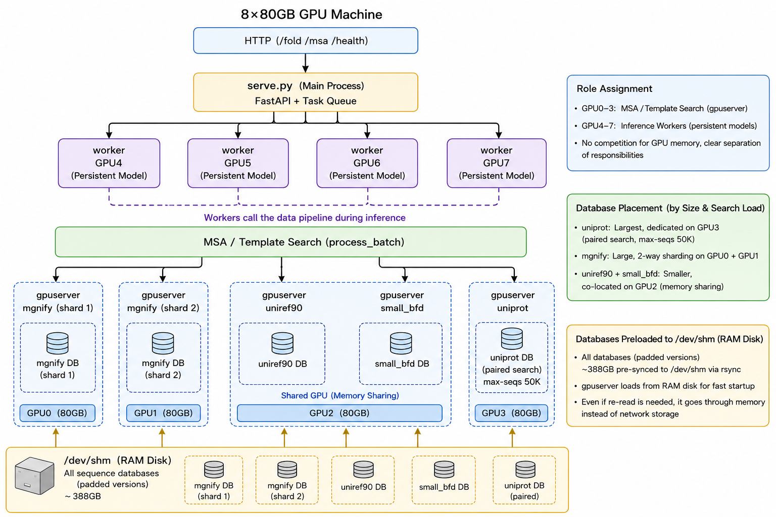
serve.py) dispatches jobs to four inference workers on GPU4 to GPU7, each holding the model weights resident. MSA/template search (process_batch) fans out to four gpuserver processes on GPU0 to GPU3, each holding one database resident in VRAM; all databases are staged on /dev/shm. (Image source: this work, based on AlphaFast.)Three decisions shape this layout. (1) Separate the MSA GPUs from the inference GPUs. GPU0 to GPU3 run the resident MSA gpuservers; GPU4 to GPU7 run the resident inference workers. Neither side competes with the other for VRAM. (2) Place each database by its size and search load. UniProt is the largest (used for pairing, with max-seqs set to 50k), so it gets a card to itself; MGnify is also large and is sharded two ways across two cards; UniRef90 and the reduced BFD are smaller and share one card. (3) Stage every database on /dev/shm (the padded versions total ~388 GB), so gpuserver loads from a RAM disk. That is fast to start, and any re-read goes through memory rather than network storage.
4. Five layers of speedup
The speedup is not one trick but five separate optimizations, each removing a different kind of repeated cost. Four of them attack the MSA stage, which is the bottleneck: keeping the database resident, putting the alignment on the GPU, batching and parallelizing the search, and caching results. The fifth keeps the inference weights resident. I'll cover the three MSA-search layers first, then the one for inference, and finally the cache that sits over all of them.
4.1 Keep the database resident in VRAM (gpuserver)
A plain mmseqs search --gpu 1 reads the target database in on every search, and for a database of hundreds of GB that load alone is on the order of minutes. gpuserver removes it: a long-lived process loads the database into VRAM once, and later mmseqs search --gpu-server 1 calls connect to it, so the cost drops from "paid on every search" to "paid once, at startup." The price is that VRAM stays occupied by the database, which is exactly why the MSA and inference GPUs have to be kept apart.
4.2 Run the alignment on the GPU (--prefilter-mode 3)
A resident database does not help if the alignment itself, gapped alignment in particular, quietly falls back to the CPU; then you get a saturated CPU and an idle GPU. As described back in Section 2, --prefilter-mode 3 keeps both the gapless prefilter and the gapped alignment on the GPU. It is easy to confirm: watch nvidia-smi during a search, and the database's card should sit near 100%.
4.3 Batch the chains and run the databases concurrently (process_batch)
The naive pipeline is serial over chains and over databases: 3 chains × 4 databases is 12 sequential searches. Both dimensions can be collapsed. Across chains, batch: pack the unique sequences of all chains in a complex into one search per database, and let the GPU process many queries at once. Across databases, run concurrently: the four databases live on different GPUs, so their searches launch at the same time, and because gpuserver keeps them resident, concurrency does not OOM from repeated loading.
A boundary worth naming. Only the GPU search is concurrent; the
result2msastep right after it (turning hits into a3m) is CPU-bound and scales poorly. Moving the four-database search from serial to concurrent dropped cold MSA only from ~100 s to ~95 s (about 5%), because the real floor is CPU-sideresult2msa, which parallelism cannot remove; capping its thread count or not made almost no difference. The only levers left are loweringmax-seqs(at the cost of MSA depth) or caching.
4.4 Keep the model weights resident
This is the one layer that is about inference rather than MSA. Each inference worker builds a ModelRunner once, at startup, loads the weights into its card's VRAM, and keeps them there, so requests run inference directly and skip the several-GB weight load every time. The arithmetic is simple: N inference cards give N workers, N resident copies of the weights, and N folds in flight at once.
4.5 Cache the finished MSA per sequence
Even when the search is fast, re-running it for sequences that recur (the chains shared across a batch of related inputs) is wasted work. A cache removes that, and the only real decision is granularity. Scheme A caches the raw a3m per database (key = database + sequence), so a hit still needs parsing and cross-database deduplication, the CPU work beyond result2msa. Scheme B caches the finished MSA (key = sequence): the deduplicated unpaired/paired MSA plus templates, stored as a single JSON, so a hit pours straight back into the chain and skips search, parsing, deduplication, and templates entirely.
For an online service whose pipeline configuration is fixed (the database set, max-seqs, and deduplication never change), Scheme B is the right fit: "a sequence and its finished MSA" is a stable, cacheable product, and Scheme A's flexibility (recombinable intermediate products) buys nothing here. The gap is large:
| Cold | Warm (hit) | |
|---|---|---|
| Scheme A | ~95 s | ~1.3 s (still parses + dedups) |
| Scheme B | ~95 s | ~0.0 to 0.1 s (whole chain skipped) |
The implementation is almost free. In AF3's input JSON, each chain can be pre-filled with unpairedMsa, pairedMsa, and templates, and once pre-filled the data pipeline skips that chain's search. So Scheme B changes nothing in the pipeline; it only pours cached content into the matching chains before the request enters it, reusing AF3's own "if MSA is given, don't search" logic. The one caveat is that any configuration change (a different database, a different max-seqs, different deduplication) invalidates the cache and forces a clear, for either scheme.
This is where the section's theme lands. Caching does not lower the cold cost; it sidesteps it. A warm request skips MSA entirely, but a cold one is still floored by CPU-side result2msa at roughly 80 to 90 s. That floor is the ceiling on everything here: every layer above either avoids the MSA work or moves it onto the GPU, and what stays on the CPU is what you cannot speed up further without giving up MSA depth.
5. The service layer: designing serve.py
The full code for this section is on GitHub: v-shaoningli/alphafast-server (alphafast-serving branch). The skeleton is intentionally plain: one FastAPI main process, one worker subprocess per inference card, and a task queue between them. A request's life cycle looks like this:
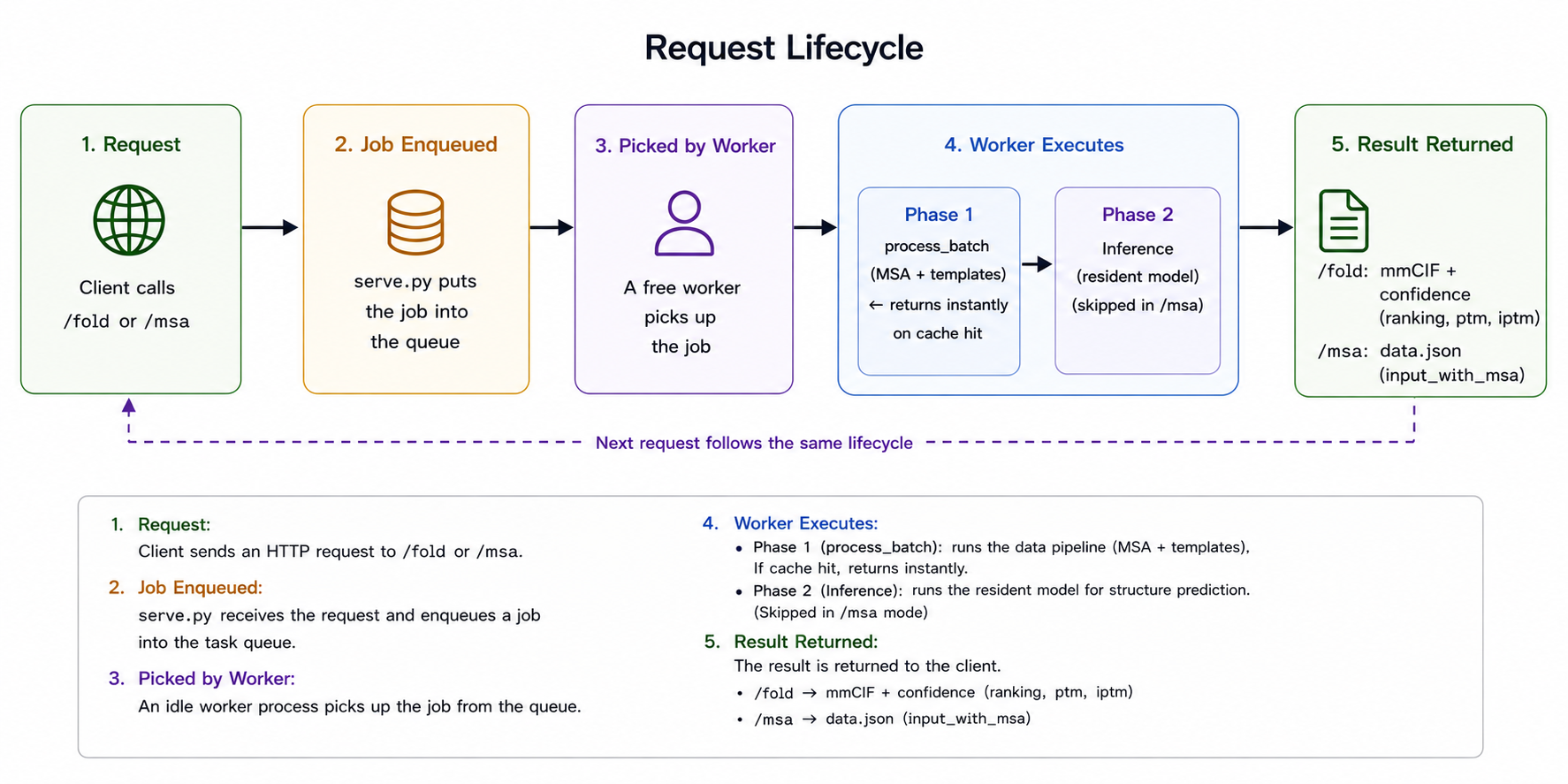
serve.py. A /fold or /msa call is enqueued and picked up by a free worker, which runs phase 1 (the data pipeline's process_batch for MSA and templates, returning instantly on a cache hit) and then phase 2 (resident-model inference, skipped in /msa mode), returning the structure plus confidence, or the MSA.The endpoints are shaped around how the service is actually used. /fold does a full fold, returning the structure (mmCIF) plus confidence (ranking, ptm, iptm). /msa searches only MSA and templates, returning a reusable data.json for users who want the MSA but not the fold; it shares phase 1 with /fold, so the two paths stay consistent. /health returns workers_ready / workers_total for liveness checks and "wait until ready." A request can also specify output_dir, letting the service write all diffusion samples to shared storage for the client to read, rather than stuffing several large cif files into an HTTP response.
One small trick on GPU mapping is worth calling out: each worker binds a single physical card via CUDA_VISIBLE_DEVICES and then treats it as "device 0" internally. The logic never has to know which physical card it is actually running on.
6. Three alignment rules for gpuserver
Wiring the client's searches to gpuserver produced two genuinely puzzling failures. One was a deadlock: GPU utilization stuck at 0%, the search hanging forever. The other was malloc(): corrupted top size, with the process crashing outright.
The root cause, in the end, is that gpuserver and client have to agree on three things exactly, or you get either a deadlock or memory corruption:
| Must match | Consequence if it doesn't |
|---|---|
--max-seqs (per-database result cap) | malloc(): corrupted top size, crash |
--prefilter-mode | inconsistent behavior, sometimes a crash |
CUDA_VISIBLE_DEVICES (the device string itself) | deadlock, GPU at 0% |
The operational key is that gpuserver discovery is keyed on (database path + CUDA_VISIBLE_DEVICES string). So whatever max-seqs a database's gpuserver was started with, the client searching that database must use the same; and the card that started a gpuserver and the client that searches it must see the same set of cards. The safest approach is to define this per-database parameter table once in the launch script and have server and client share it.
A lesson on the side: errors like
corrupted top sizeare deeply misleading. They pull you toward a sharding bug, a threading problem, or a corrupted binary. The real cause is usually just parameters that don't line up.
7. Performance numbers (8×A800)
With all of the above stacked together, here are the measured numbers for one concrete target, PDB 7YV1:
| Scenario | MSA | Inference | Total |
|---|---|---|---|
/fold, cold (new sequence) | ~95 s | ~134 s | ~230 s |
/fold, warm (sequence cached) | ~0 s | ~134 s | ~134 s |
/msa, cold / warm | ~95 s / ~0 s | n/a | ~100 s / ~1 s |
A few observations. The cache is the biggest lever: a warm request erases the entire MSA stage and leaves only inference. In batch settings, where a group of inputs shares most of its chains, the shared chains hit the cache and only the changed chain is searched. Multiple cards give parallelism: four inference workers mean up to four folds running at once, one card each. On capacity, the MSA gpuservers are concurrency-safe; the UniProt card's peak VRAM is essentially constant (results stream back to the host rather than piling up in VRAM with batch size), and the load cost sits on CPU-side result2msa, not on the GPU. As for the floor that won't move: cold MSA's result2msa (CPU) is a hard floor at roughly 80 to 90 s, reducible only by caching (the warm path) or by lowering max-seqs.
8. Takeaways
- Persistence is really about paying one-time costs once. Databases, weights, and environment are paid once; each request then pays only the increment. The test for whether to go persistent is simply whether your workflow folds the same kind of input repeatedly.
- Speedups come in layers, each owning one stage. Resident databases save loading; alignment-on-GPU saves the CPU; batching plus concurrency saves serialization; resident weights save loading again; caching saves repetition. Only by understanding each layer's boundary do you know where the ceiling is. Here, it is CPU-side
result2msa. - Match cache granularity to the use case. For a fixed-configuration service, caching the finished MSA (sequence-level) is cheaper and more direct than caching intermediate products (database-level).
- gpuserver parameters must align between server and client.
max-seqs,prefilter-mode, and the visible cards all have to match, or the crash message will mislead you.
In the end, persistence plus caching pull the marginal cost of folding the same target repeatedly down to inference only. For the many variant-scanning and redesign workflows in structural biology, turning folding into a service is a one-time investment well worth making.
Acknowledgements / Credits
This post is, at bottom, an engineering exercise in "servicizing" the open-source work below. Credit for the core models and algorithms goes to their authors:
- AlphaFast (RomeroLab): the thing actually deployed here. It wires MMseqs2-GPU into the AF3 data pipeline, giving the order-of-magnitude MSA speedup; the resident
gpuserver, prefilter-mode 3, and batched/concurrent search all come from it. - AlphaFold3 (Google DeepMind): the underlying structure-prediction model and data pipeline. Please respect the terms on its weights and code.
- MMseqs2 / MMseqs2-GPU (Steinegger lab & Söding lab): the GPU-accelerated homology search engine at the root of the MSA speedup.
My own contribution is only at the deployment and service layer: the split of roles across GPUs, the persistent-service and cache design, the gpuserver alignment rules, and these field notes. Everything about the models and the search algorithms themselves belongs to the projects above.
References
- Abramson, J., Adler, J., Dunger, J. et al. Accurate structure prediction of biomolecular interactions with AlphaFold 3. Nature 630, 493-500 (2024). https://doi.org/10.1038/s41586-024-07487-w
- Steinegger, M. & Söding, J. MMseqs2 enables sensitive protein sequence searching for the analysis of massive data sets. Nature Biotechnology 35, 1026-1028 (2017). https://doi.org/10.1038/nbt.3988
- Kallenborn, F., Chacón, A., Hundt, C., Sirelkhatim, H., Didi, K., Cha, S., Dallago, C., Mirdita, M., Schmidt, B. & Steinegger, M. GPU-accelerated homology search with MMseqs2. Nature Methods 22, 2024-2027 (2025). https://doi.org/10.1038/s41592-025-02819-8
- Perry, B.C., Kim, J. & Romero, P.A. AlphaFast: High-throughput AlphaFold 3 via GPU-accelerated MSA construction. bioRxiv (2026). https://doi.org/10.64898/2026.02.17.706409. Code: https://github.com/RomeroLab/alphafast
- Suzek, B.E., Wang, Y., Huang, H., McGarvey, P.B., Wu, C.H., the UniProt Consortium. UniRef clusters: a comprehensive and scalable alternative for improving sequence similarity searches. Bioinformatics 31(6), 926-932 (2015). https://doi.org/10.1093/bioinformatics/btu739
- Richardson, L., Allen, B., Baldi, G. et al. MGnify: the microbiome sequence data analysis resource in 2023. Nucleic Acids Research 51(D1), D753-D759 (2023). https://doi.org/10.1093/nar/gkac1080
- Steinegger, M., Mirdita, M. & Söding, J. Protein-level assembly increases protein sequence recovery from metagenomic samples manyfold. Nature Methods 16, 603-606 (2019). https://doi.org/10.1038/s41592-019-0437-4 (the Big Fantastic Database, BFD)
- The UniProt Consortium. UniProt: the Universal Protein Knowledgebase in 2023. Nucleic Acids Research 51(D1), D523-D531 (2023). https://doi.org/10.1093/nar/gkac1052